metagenome-assembly-workshop
Metagenome Assembly from Long Reads
In this workshop we will assemble a mock metagenome from the following species
| Proportion of Reads | Species | Accession | Number of Chromosomes | Size | GC Content |
|---|---|---|---|---|---|
| 44.5 | Geitlerinema sp. PCC 7407 | ASM31704v1 | 1 | 4.7Mb | 58 |
| 30 | Vibrio alfacsensis | ASM1967048v1 | 2 | 5.3Mb | 44 |
| 7.5 | Vibrio algicola | ASM960176v2 | 3 | 3.5Mb | 42 |
| 15 | Desulfovibrio sulfodismutans | ASM1337645v1 | 2 | 4.4Mb | 63.5 |
| 3 | Winogradskyella schleiferi | ASM1339465v1 | 1 | 4.6Mb | 34.5 |
We will proceed through a full metagenomic analysis consisting of the following steps
- Assembly
- Basic assembly QC and contig filtering
- Binning
- Bin assessment
- Taxonomic classification of bins
Setup
Data for the workshop is provided in a folder on the rstudio server
called metagenome_assembly in your home directory.
Look inside this folder with the ls command
ls -R metagenome_assembly
The raw_data folder contains reads that will be used for our assembly.
All of the other folders are empty. We will use those to contain work
for each step of our analysis.
Assembly
Assuming that we are satisfied with the overall quality of our reads the first step is to assemble them. We will use flye for this task because it is probably the best assembler for long-read metagenome data.
Change to the flye directory in our project folder
cd metagenome_assembly/flye
Run flye.
flye --nano-hq ../raw_data/sim.fastq.gz --threads 8 --out-dir mock --meta
Once finished, outputs from flye will be available in the directory
mock. The key output files are;
| File | Description |
|---|---|
| assembly.fasta | The actual assembled contigs |
| assembly_graph.gfa | Representation of the assembly graph in gfa format. |
| assembly_graph.gv | Assembly graph in graphviz format |
| assembly_info.txt | Table of information on each contig |
Exercises
- What is the size and coverage of the largest contig in the assembly?
- Visualise the assembly using bandage
- Based on coverage and size can you guess which species the four largest contigs correspond to?
Calculating GC content
Before moving onto more formal binning analysis it is worthwhile quickly inspecting some more properties of our assembly.
Firstly we will calculate GC content for each of our contigs. This could be used to refine the rough contig groupings we made using Bandage
Switch to the filter directory
cd filter
Create a new file plain text file called gc.awk inside this directory.
Open this file and copy-paste the following awk script into it.
# Bioawk script for calculating gc
BEGIN {
    OFS="\t"
}

{
    l=length($seq)
    ngc=gsub("[cgCG]","",$seq)
    nat=gsub("[taTA]","",$seq)
    lend=length($seq)
    print $name,l,ngc/(ngc+nat)
}
After you have saved the file you should now be able to run it as follows
cat ../flye/mock/assembly.fasta | bioawk -c fastx -f gc.awk > assembly.gc.tsv
Now take a look at the GC content values for the top 10 largest contigs
cat assembly.gc.tsv | sort -n -k 2 -r | head
Compare these values with the expected GC content from our mock community. Considering both GC content and coverage, does this affect your ideas about how these contigs should be assigned to taxa?
Now let’s create some plots in R to explore the GC and coverage of contigs in a slightly more general way.
First read the gc and assembly_info datasets.
library(tidyverse)
gc <- read_tsv("filter/assembly.gc.tsv",col_names = c("#seq_name","length","GC"))
info <- read_tsv("flye/mock/assembly_info.txt")
Join them together
gc_info <- info %>%
  left_join(gc)
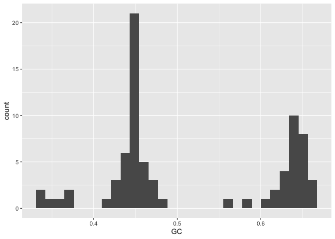
A histogram by GC content shows several peaks, probably corresponding to major groupings of taxonomically distinct lineages within the data.
gc_info %>%
  ggplot(aes(x=GC)) + geom_histogram()
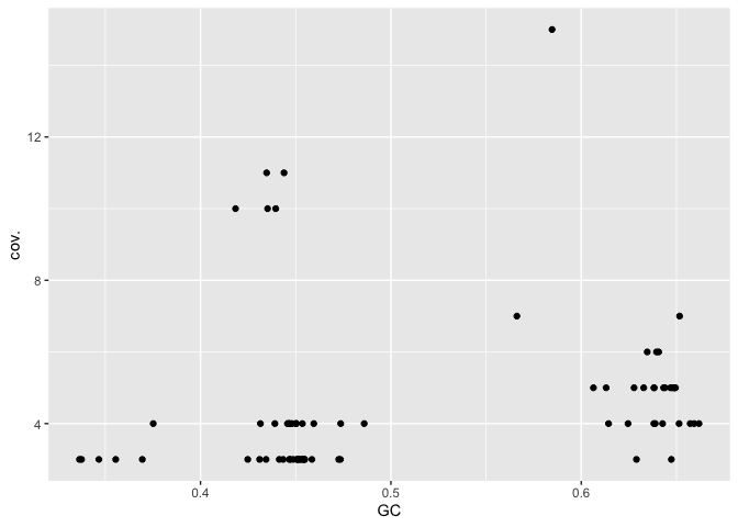
A plot of GC vs coverage helps to identify clusters that have similar values for both these parameters.
gc_info %>%
  ggplot(aes(x=GC,y=cov.)) + geom_point()
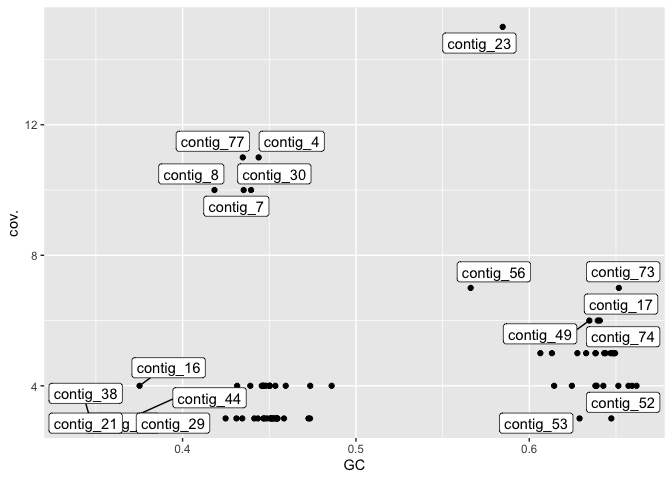
Adding labels allows us to look at the contigs with highest coverage and compare these with the contigs in bandage.
library(ggrepel)
gc_info %>%
  ggplot(aes(x=GC,y=cov.)) + geom_point() + geom_label_repel(aes(label=`#seq_name`))
Binning
One of the most challenging tasks in metagenomic assembly is separating sequences from the many different organisms that were present in the sample. There are many approaches to this and many different tools. Broadly speaking tools fall into two categories;
- Read binning tools which group the raw (unassembled) reads
- Contig binning tools which group assembled contigs
In both cases the resulting outputs are “bins” each of which will contain multiple distinct sequences (reads or contigs) that come the same organism. It is important to acknowledge that binning is a very difficult problem and the results from binning tools often contain errors such as;
- Placing two sequences together when they come from different taxa (leads to “contamination”)
- Failing to group sequences that come from the same taxon (lead to fragmentation)
We will perform contig binning here since we have long-reads and can rely on metaFlye to do a good job of assembling high quality contigs from a mixed collection of reads.
Firstly we will use the program metabat2. This program tries to group
contigs based on nucleotide composition and read coverage.
For simplicity and speed we will use coverage information already
calculated by flye and provide this to metabat.
First prepare an input file summarising read depth information for all contigs
cd metabat
cat ../flye/mock/assembly_info.txt  | grep -v '#' | awk '{OFS="\t";print $1,$3}' > depths.txt
Next we need to create a new version of the assembly file in which the
contigs have the same order as those in the depths.txt file.
cat depths.txt | awk '{print $1}' | xargs samtools faidx ../flye/mock/assembly.fasta > assembly_ordered.fasta
Finally, run metabat as follows
metabat -i assembly_ordered.fasta -a depths.txt --cvExt -o bins/metabat --seed 5
The bins directory will contain multi-fasta files with each of the
bins inferred by metabat. To quickly inspect which contigs were grouped
into which bin we can just use a grep command like this
grep '>' bins/*
You can see here that metabat has grouped contigs into 7 bins (exact
numbers can vary from run to run which is why we used the --seed
argument above). If you compare the contigs in these bins with those
shown in bandage you can see that the largest and highest coverage
contig has not been included. Other than this some of the other bins to
seem to make some sense. For example, bin number 4 includes contigs 4
and 30, 7 and 8 all of which have a similar GC content and coverage.
Consolidation of bins with large unbinned contigs
In this step we will collect bins created by MetaBAT and also include any large contigs that were skipped by the binning step.
First switch back to the filter directory and make a subdirectory
called long_contigs
cd filter
mkdir -p long_contigs
The following code will collect the longest 20 contigs and place each
into its own fasta file within the long_contigs directory
while read contig;do
    echo $contig;
    samtools faidx ../flye/mock/assembly.fasta $contig > long_contigs/$contig.fasta;
done <  <(cat ../flye/mock/assembly_info.txt | grep -v 'seq_name' | sort -n -k 2 -r | head -n 20 | awk '{print $1}')
There is quite a bit going on in this code. Before running it let’s break it down and see how it works
First let’s just focus on the bash while loop. A much simpler loop would be
while read item;do
  echo $item
done < <(echo "1 2")
Now let’s look at what is “feeding” the loop. It expects to be reading a
file line by line. We don’t actually have a file but we can trick bash
into thinking we have one by using the construct <(). Text output
generated by a command inside the brackets is treated as if it were in a
file.
Let’s examine the code we are using to generate our list of contigs
cat ../flye/mock/assembly_info.txt | grep -v 'seq_name' | sort -n -k 2 -r | head -n 20 | awk '{print $1}'
Break this down by removing the pipes and gradually adding them back
Finally we can look at the command used to extract contigs
samtools faidx ../flye/mock/assembly.fasta contig_1
Now we are in a position to identify the long contigs that were not otherwise included in our MetaBAT bins.
# Make a sorted list of contigs in metabat bins
grep '>' ../metabat/bins/metabat.[0-9]*.fa | sed -E 's/.*(contig_.*)/\1/' | sort > metabat_contigs.txt

# Make a sorted list of long contigs
cat ../flye/mock/assembly_info.txt | grep -v 'seq_name' | sort -n -k 2 -r | head -n 20 | awk '{print $1}' | sort > long_contigs.txt
Use the comm command to print contigs present in long but not
present in metabat.
comm -13 metabat_contigs.txt long_contigs.txt > missing_contigs.txt
Check bin quality with checkM
Switch to the checkm directory
cd checkm
Collect bins from metabat and combine with long contigs
mkdir bins
cp ../metabat/bins/metabat.[0-9]*.fa bins/

while read contig;do
    cp ../filter/long_contigs/${contig}.fasta bins/${contig}.fa
done < <(cat ../filter/missing_contigs.txt)
Take a look in your bins folder. It should contain some files with
names like metabat.[0-9].fa and others like contig_23.fa.
Now run the checkm workflow. This could take quite a while.
checkm lineage_wf bins out -t 10 -x fa -f checkm_results.txt
Once checkm has finished take a look at the results file,
checkm_results.txt. It provides a summary of results for each of the
bins. This includes
- Marker Lineage: An approximate taxonomic classification. This is used by checkM to determine which marker genes to use for completeness and contamination checks
- # genomes: number of reference genomes used to infer marker set
- # markers: number of inferred marker genes
- # marker sets: number of inferred co-located marker sets
- 0-5+: number of times each marker gene is identified
- Completeness: estimated completeness
- Contamination: estimated contamination
- Strain heterogeneity: estimated strain heterogeneity
Perform taxonomic assignment
Change to the gtdbtk directory
cd gtdbtk
Make a symbolic link to the bins and call it genomes
ln -s ../checkm/bins genomes
Run gtdbtk. This will take a while
conda activate gtdbtk-2.1.1
gtdbtk classify_wf -x fa --cpus 10 --genome_dir genomes --out_dir out
Once it has finished running you can find the final output table in
out/classify/gtdbtk.bac120.summary.tsv
Take a look at this table
head -n 2 out/classify/gtdbtk.bac120.summary.tsv
An easier way to look at it might be to load it into R
gtdbtk <- read_tsv("gtdbtk/out/classify/gtdbtk.bac120.summary.tsv")
There are many columns in this output, however, the key one is
classification. You should see from this that only four of the bins
were classified. Looking at the classifications though we can see that
they are very close to our reference genomes.
Further Quality Assessment with MetaQuast
MetaQuast provides several useful visualisations for assessing metagenome assembly quality. In this case since we know the reference genomes of all members of our community we can use it to see how well our assemblies match those.
cd metaquast

ln -s ../gtdbtk/genomes .
ln -s ../raw_data/refs .
Run metaquast. This will download each of the reference genomes from NCBI and perform alignments between each of the bins and these genomes.
metaquast.py genomes/*.fa -o out --references-list refs/references.txt -t 4
When metaquast is finished running you can find an html report in the
output folder out/report.html. This is a little confusing but it
essentially confirms that two of our genomes (those with the most
coverage) are assembled very well.
Optional
Alternative binning program
An alternative binning option is metabinner. This is a much newer program that uses a greater suite of information when performing binning. It is also very new, a little hard to use, and much much slower than metabat.
When performing binning for your own projects you could explore a range of tools. Your goal should be to obtain bins with high checkM scores (see below) and that are supported by multiple tools.
The code below shows how to run metabinner. Please DO NOT run this during the day when we are in the workshop as it will use up too much CPU on the server. Try it yourself after the workshop is complete.
conda activate metabinner

cd metabinner

cp ../metabat/depths.txt
cp ../metabat/assembly_ordered.fasta

/opt/miniconda3/envs/metabinner/bin/scripts/gen_kmer.py assembly_ordered.fasta 1000 4

run_metabinner.sh -t 10 -a $(pwd)/assembly_ordered.fasta -o $(pwd)/mbout2 -d $(pwd)/depths.txt -k $(pwd)/assembly_ordered_kmer_4_f1000.csv -p /opt/miniconda3/envs/metabinner/bin